Some visual intuition for 2D Fourier transforms
Improving by blurring
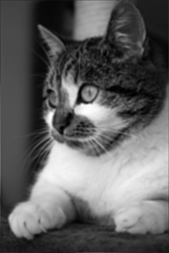
Let’s say we have a image of a cat and we want to blur it a bit


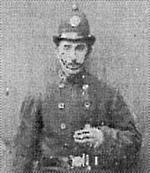
That’s pretty cute, but you may not need blurred cat images so often. However there are also more useful things we can do using the exact same method. This here is Constable Sinclair Tait of the Inverness-shire Constabulary
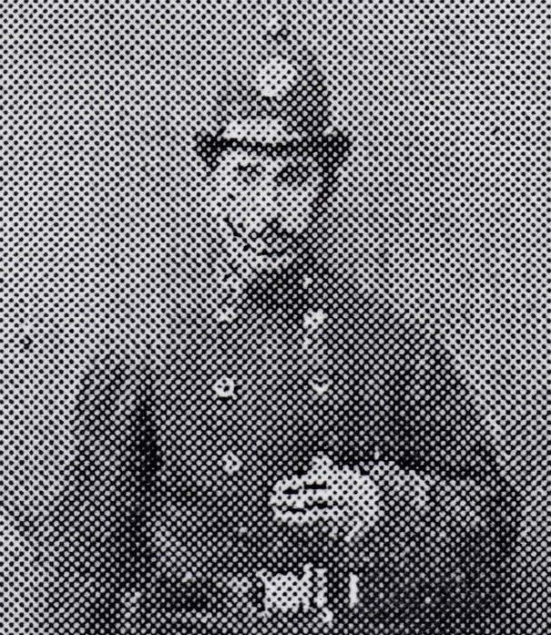
Many things can be said about Mr. Tait, which you can read a lot more about on Dave Conner’s Flickr, but he certainly hasn’t been preserved all that well. The interesting thing is that by using the exact same method as for blurring a cat we can bring some life back to our constable:

That’s pretty neat, and, some would argue, more useful than blurred cats. So how does it work?
The Fourier transform
Both the cat blurring and constable reconstruction is done by applying a low-pass filter to the images, or, in other words, by removing high frequencies.
The way we go about is by a Fourier transformation of our image. I will not go into too many details of exactly how or why it works in this post - for now all we need to know is that any1 function or signal can be expressed as a sum of sine and cosine functions to arbitrary precision.
How does this help us blur cats? Consider this illustration by Lucas Barbosa of a 1D function being decomposed into it’s frequency components
.gif)
Here a square wave function \(f\) is decomposed into a range of sine and cosine functions each multiplied by a constant \(a_n\) or \(b_n\) (their amplitude) and each with a different frequency (here proportional to \(n\)) - if each of these individual sine and cosines were to be added together the result is again the original function \(f\). We are essentially seeing \(f\) being split up into its frequency components, and the function \(\hat{f}\) shows us how large each component is.
This is essentially what the Fourier transform does - it tells us which frequencies a function or signal consists of and how strong they each are. In other words, if our signal is in “real space” we can transform it to “frequency space”.
Notation and an important property
Applying the Fourier transform can be denoted as \(\mathcal{F}\left\{f\right\} = \hat{f}\), where \(f\) is transformed into \(\hat{f}\). Importantly we can directly recover our original function with the inverse Fourier transform, \(\mathcal{F}^{-1}\{\hat{f}\} = f\). For disctrete (digital) signals such as images we typically use a numerical version called a Fast Fourier Transform. For our use in this blog post we consider them equivalent, and I will use “the FFT” in some places to refer to the result of a transform on an image.
A very useful fact about the Fourier transformation is its linearity. This means that the Fourier transform of a sum of functions can be expressed as a sum of individual Fourier transforms on each function: \(\mathcal{F}\left\{f_1 + f_2 \right\} = \mathcal{F}\left\{f_1\right\} + \mathcal{F}\left\{f_2\right\}\)
We are going to leverage this to our advantage.
Frequencies in an image
Let’s experiment a bit and create a little 2D image. Here \(x\) and \(y\) goes from \(0\) to \(2\pi\) (i.e. one full period of a trigonometric function) and we plot the function \(f_1 = \cos (4x)\)

The FFT of this simple cosine looks like this
Two dots spaced equally apart from the image center - these are the frequency components of our image, and since our image is a “pure” cosine the frequency is very well defined. The reason there are two dots instead of just one, despite having just one frequency, is beyond the scope of this post. Just know that a Fourier transform of a real valued signal gives a symmetric and complex valued result, meaning each pixel in our image is a complex number, \(z=a+ib\). The two dots represent exactly the same frequency and are each others complex conjugate2. When I “show the fourier transform” what I am actually showing is the absolute value of each point \(\lvert z \rvert\)3.
Let’s try with a higher frequency and see how \(f_2 = \cos(8x)\) and its fourier transform looks


Again two dots centered around the middle, but now they are further apart. The last bit is important; higher frequencies are further away from the center in the FFT image.
We can also add the two images together, so we’re now seing \(f_3 = \cos(4x) + \cos(16x)\)

Then we have two sets of dots, exactly corresponding to the two frequencies we are visualising. And importantly, even though everything is muddled together in “real space”, we still se everything distinct in “frequency space”.
If we turn the picture by plotting \(f_4 = \cos(4y)\) we also turn the arrangement of dots


Again we can add the pictures together, i.e. our image now shows \(f_5 = \cos(4x)+\cos(8x)+ \cos(4y)\)
And again we see two distinct peaks for each frequency in our image.
Filtering with a mask
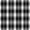
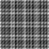
Let’s freshen things up a bit and try with a whole bunch of frequencies
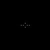
If you look closely you can see that our previous image with \(f_5\) is actually contained in the one above. It’s quite difficult to see in real space but in the FFT the dots from before a still clearly distinct from all the new ones.
Let’s recover them!
Since all the unwanted frequencies are higher than the ones we want, we can do so with a high-pass filter. A simple way of doing this is to just set all frequencies above a certain treshold to \(0\). Remember that in the FFT the frequency is proportional to the distance from the center. This means we will need a circular mask, where white pixels are \(1\) and black are \(0\).

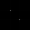
Now we can apply the mask to the FFT image by multiplying them together (both real and imaginary parts). This way each pixel with a \(0\) in the mask becomres \(0\) in the FFT, and \(1\)’s in the mask simply keep their value. This results in the following

That should seem familiar. The lines crossing in the center are artifacts from discretization of the higher frequencies, but they don’t matter to omuch now. We can now do an inverse Fourier transform and recover our image!
And we’re back to how we started!
Blurring the darn cat
This brings us back to the cat. Let’s see it again along with its fourier transform4.
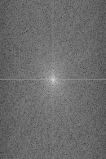
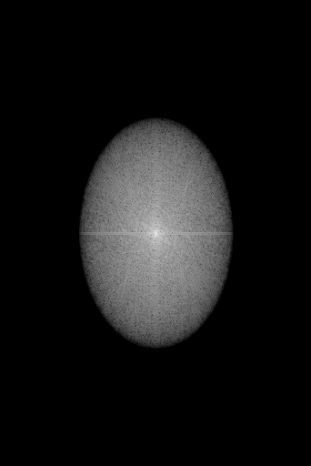
As there are not many well defined frequencies in the picture we don’t have the same well defined spots as before. Let’s do the same as we did to that previous image and cut off some higher frequencies (aka. use a low pass filter). As before we create a mask and apply it to our image

The mask is made from a Tukey window which has tapered edges to avoid edge artifacts which would appear from a sudden frequency cutoff. There are many types of window functions to use (you can even make your own!). I chose Tukey somewhat arbitrarily - we’ll save the specifics for another post.
We can increase or decrease the diameter of our filter (or window) which will in turn increase or decrease the cut off frequency and thus the sharpness of our image:


Restoring the Constable
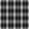
Using what we have now (hopefully) learned, we return to Mr. Tait and his Fourier transform
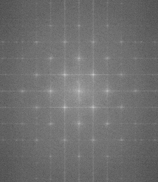
The dots are back! Why is that? As we saw earlier, a well defined frequency in an image leads to a well defined point in the FFT. The dots which were used to print Mr. Taits portrait are very evenly spaced and can be apparently represented well by a limited, fairly well defined set of frequencies. This is good news for us if we want to restore his image as we then only need to block fairly specific frequencies.
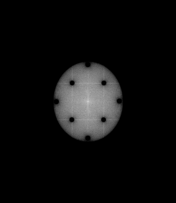
We can begin with the easy way - just cut off all frequencies above a certain point which contains the dots:

Not a bad start!
But we may want to keep some information in the higher frequencies. We can basically do whatever we want with the FFT image. Instead of simply cutting off everything above a certain frequency (low-pass filter) we’ll try to just blot out the dots and keep everything else.
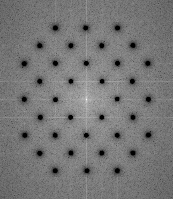
We create a new mask, this time much smaller than the picture and inverted compared to before

This time we have \(0\)’s in the center and \(1\)’s at the edge, so when we multiply this onto our image we can “erase” certain points. From this we create a larger mask which we can apply to the FFT of the constable

The inverse transform gives us the filtered constable

Not perfect.
You may be thinking that the improvement was not very significant compared to just the low-pass filter, and you would actually be correct.
The reason is there cannot be any details “between the dots” in the original image. In other words, as all information in the original image is encoded purely by the dots themselves, there shouldn’t be any additional information with higher frequency than those, and when we cut away higher frequencies we don’t lose image information. However there may be additional details from the digitalisation (dust, markings, etc.) which could be interesting for some applications. There are also some artifacts around the edges, which I have not accounted for, seen as vertical and horizontal streaks in the FFT, but that is maybe food for a future blog post.
Let us combine the two methods and do both a notch filter and low-pass filter
Our constable has now reached his final form:
There are many other techniques that can be used for this kind of image reconstruction, but it is at least interesting to see how much you can do with a fairly straight forward method.
The principles we have seen and the intuition gained from playing with transforming images can carry over and be of great help in many other areas of science and physics, including understanding of lenses, diffraction gratings, crystallography and many other (some of which I hope to write more about here!)
Hope you enjoyed reading!
-
There are exceptions, but most reasonably well-behaved functions one might normally encounter in the physical world (and the mathematics describing it) has a Fourier transform. There is a bit more on that on this Stackexchange question. ↩
-
complex conjugation is fancy speak for “the \(i\) changes sign” in a complex number. Thus the complex conjugate of \(a + ib\) is just \(a - ib\). ↩
- \[\lvert z\rvert = \sqrt{a^2 + (i b)^2} = \sqrt{a^2 + b^2}\]
-
I am now displaying the logarithm of the value of each pixel now, i.e. \(\log\left(\lvert z \rvert\right)\) for all pixels, as the main peak would dominate everything in the image. With the logarithm lower valued pixels are enhanced and easier to see. ↩