Visualizing the magnetic field of nanoparticles - Fundamentals
This is the first of two posts - the second on reconstructing holograms using Python can be found here.
When learning about magnets and magnetic fields, you have probably seen visualizations similar to these1 which represent how the magnetic field extends outside a rectangular magnet

The left represents how iron filings agglomerate when sprinkled around a magnet as they roughly align to the magnetic field, a common method to directly “see” the magnetic field around larger magnets. In the middle the magnetic field is represented with a series of magnetic field lines which are drawn along lines of constant field strength, while the rightmost image shows how an array of freely rotating magnets (e.g. compasses) would align themselves in the same magnetic field.
This is usually presented for magnets large enough hold in your hand, but it is actually possible to directly measure the magnetic field all the way down at the nano scale in a Transmission Electron Microscope or TEM, just like this:
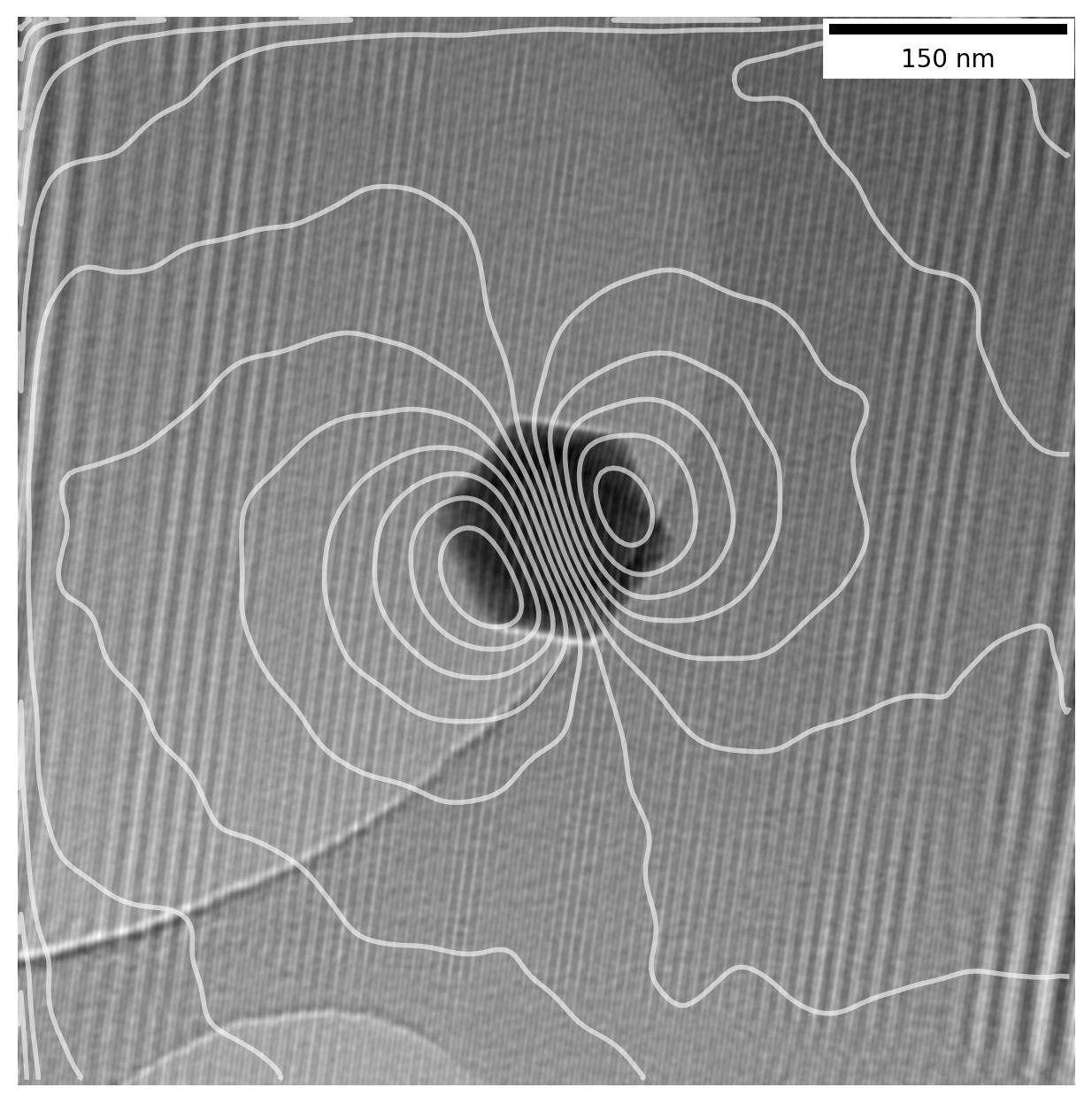
The above image shows a magnetite nanoparticle around 90 nm wide where the contour lines represent the magnetic field around the particle as measured directly in the microscope. Iron filings and tiny compasses work great for magnets large enough to handle, but what do we do when working on the nanoscale?
Below i will explain a method known as Off-Axis Electron Holography and how it can be used to measure and visualize the magnetic field around magnetic nanoparticles in the TEM to make images like the above. Much of what follows is based on this book chapter2 on electron holography of magnetic materials which I recommend reading if you are interested in the subject.
The data shown was acquired as part of my bachelors thesis3 at DTU Nanolab (previously Center for Electron Nanoscopy) several years back. I recently went back to revisit the subject and redo (and improve) in Python out of curiousity and decided do this writeup to share with anyone why might be interested.
This post is part one of two and covers some TEM fundamentals and relevant mathematics. For numerical calculations, take a look at part two where we reconstruct holograms using Python.
Very brief intro to the TEM
A Transmission Electron Microscope in conventional operation is very similar to a typical optical microscope, but instead of using light waves we use a beam of electrons. Since electron waves generated at high voltages have a much shorter wavelength than visible light, we can use it to see much smaller things. As an example, blue light has a wavelength around \(400 \unit{nm}\), while an electron will have a wavelength around \(0.0025 \unit{nm}\) at \(200 \unit{kV}\) acceleration voltage – for reference a hydrogen atom has a diameter of around \(0.01 \unit{nm}\)4.
The diagram below shows a simplified schematic of a TEM in bright field (BF) mode, where an electron gun at the top provides a beam of coherent electrons which are condensed to a uniform plane wavefront before passing through a sample. After this the beam is focused, various apertures can be inserted, and the image is formed in the image plane on the bottom, where we place 2D detector to save the image.

Unlike in the optical microscope, the lenses are not made from glass or any physical material. Instead, we use magnetic lenses to focus the electron beam – Essentially a symmetric bunch of coils with adjustable current going through them to create a magnetic field. The reason we can manipulate the electrons with magnetic fields is due to the Lorentz force.
\[\vec{F} = q \, \vec{v}\times\vec{B}\]With a strong field of a certain shape we can use this to focus our electron beam. This is also the reason we are able to visualise the magnetic field of a sample when using electrons, as the field around a magnetic particle deflects the electrons slightly and change their phase.
I am barely scratching the surface of the subject for the sake of brevity - have a look at the very detailed and pedagogical DoITPoMS from the University of Cambridge on the TEM if you want more details.
Electron beam as a wavefunction
Mathematically we can describe the electron beam at any point \(\vr\) in the image plane as a plane wave with amplitude \(A(\vr)\) and phase \(\phi(\vr)\) in a complex exponential phase term
\[\psi(\vr) = A(\vr)e^{i \phi(\vr)}\]In typical operating conditions, when recording the image on a detector the phase information is lost as the intensity distribution is the absolute square of the wavefunction, where the conjugated exponential terms cancel out
\[I(\vr) = \left| \psi(\vr) \right|^2 = \left[A(\vr)e^{i \phi(\vr)}\right]\left[A(\vr)e^{-i \phi(\vr)}\right]= A(\vr)^2\]In other words we’re only recording the square of the amplitude of the wave, which simply tells us how many electrons reached each pixel on the sensor, regardless of their phase. This is plenty for most uses, but in our case we actually need to know the phase of the electrons.
When an electron wave passes through a sample the phase \(\phi\) of the wave will experience a phase shift. For thin magnetic samples we can express the phase shift at a given point \(\vr\) after passing through a sample as the sum of an electric and magnetic contribution
\[\phi(\vr) = \phi_e(\vr) + \phi_m(\vr)\]\(\phi_e\) arises from the electron beam intereacting with the electrons in the sample, while \(\phi_m\) depends on the in-plane component of the magnetic field from the sample due to the Lorentz force. We note that since the force is proportional to the cross product \(\vv\times\vB\), the moving charges are only affected by the components of the B-field orthogonal to the movement direction. Since the electrons are moving from the top and down into the sample they will thus only be affected by the in-plane component of the B-field. If we imagine a magnetic field pointing directly upwards from the sample, parallel to the movement of electrons there would be no phase shift, while a field perfectly orthogonal, along the sample plane, would show up fully in the phase shift.
The phase shift \(\phi_m\) is thus our key to imaging the magnetic field of our particles, and we need to figure out how to record it. As luck would have it there are workarounds for this problem.
Holography in the electron microscope
In case you are wondering, holo graphy comes from Greek and can be translated as whole drawing - in microscopy and this often refers to the fact that holographic methods preserve the phase. The “whole” in cool shiny 3D holograms on old CD’s, toys, credit cards etc. refers to the fact that they capture the “whole” three dimensional scene.
The challenge for us is to find a way to make sure the phase information of our electron wave is not lost as we record it on the detector. Below is a very simplified diagram of a TEM in a setup used for a method called Off-Axis Electron Holography.
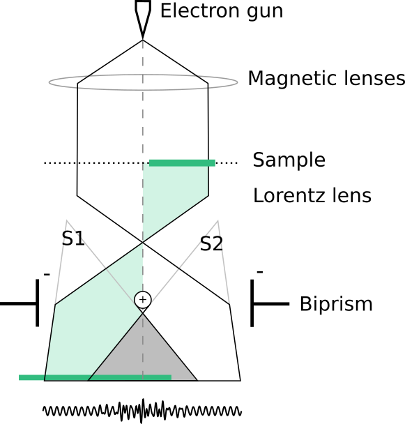
The green part of the beam which passed trough the sample we’ll call \(\psi_s\), and the other half which goes unhindered through the vacuum is our reference wave, \(\psi_r\).
Like before we generate a coherent plane wave of electrons, but now we only send part of it through the sample (green part). Further down, after the objective lens5, is the key part of the setup: the biprism. It is simply a wire going all the way through the middle of the electron beam with a plate on each side along the length of the wire outside the beam. When applying a positive charge to the beam and negative charge to the plates the electrons are repelled by the plates and attracted to the wire.
So we have essentially split the whole wavefront in two parts which we can bend towards each other causing them to overlap, and this is where the magic happens. When two coherent (in-phase) plane waves meet each other at an angle a sinusoidal interference pattern will appear as illustrated in the bottom of the diagram and can be recorded with out image sensor. The pattern is highly sensitive to small differences in phase between the two waves and will thus have information relating to \(\phi_e\) and \(\phi_m\) embedded in it.
So how do we extract the phase?
Mathematics of the phase retrieval
Let’s formalise a bit on what was described above.
Contributions to the phase shift
For a sample with no external charge distributions or external electric fields, the electrostatic contribution to the phase shift can be expressed in terms of a mean inner potential \(V_0\) which is assumed constant throughout the sample.
\[\phi_e(x,y) = C_E V_0 t(x,y)\]where \(C_E\) is a constant dependent on the microscope acceleration voltage6 and \(t(x,y)\) the thickness profile of the sample projected in the beam direction.
The magnetic phase shift can be expressed as
\[\phi_m(x,y) = -\frac{e}{\hbar} \int A_z(x,y,z) \,dz\]where \(A_z\) is the magnetic vector potential, specifically the component parallel to the electron beam direction. The gradient of the magnetic phase then gives us a direct relationship to the B-field form the phase shift
\[\nabla \phi_m(x,y) = \frac{e}{\hbar}\begin{bmatrix}B_y^p(x,y)\\\; -B_x^p(x,y) \end{bmatrix}\]where \(B^p\) is the total projection of the B-field components perpendicular to electron beam direction through the sample area
\[B^p(x,y) = \int B(x,y,z)\,dz\]As such, the phase shift of the electron beam after passing through a sample can be described as
\[\phi(x,y) = \phi_e(x,y) + \phi_m(z,y)\]Our goal now is to extract just the magnetic phase shift \(\phi_m\) of the electron beam and we need to get rid of \(\phi_e\) in some way.
If we can exactly reverse the magnetic field of our particle, the magnetic phase shift will also be reversed from \(\phi_m\) to \(-\phi_m\) while \(\phi_e\) is unchanged. In the TEM this can be done by applying a strong magnetic field in one direction, record an image, then apply a strong field in the opposite direction to reverse the magnetisation of the particle, and record another image.
We can then record two images where the magnetisation of the particle is exactly reversed between them and then subtract the phase shifts. Then \(\phi_e\) cancels out and leaves just the magnetic information
\[\phi_{\mathrm{rev}} = \phi_1 - \phi_2 = (\phi_e + \phi_m) - (\phi_e - \phi_m) = 2\phi_m\]Now we just remember to divide by 2 and we have our magnetic phase shift!7
Preserving the phase information
Remembering that the electron beam at a given point \(\vr\) in the image plane can be described as a wavefunction \(\psi_i(\vr) = A_i(\vr) e^{i\phi(\vr)}\), we now introduce a plane reference wave that only passes unhindered through vacuum
\[\psi_r(\vr)=A_r(\vr)e^{i2\pi \vq_c\cdot \vr}\]with \(\vq_c\) being a two-dimenstional reciprocal space vector determining the tilt of the reference wave. This is what we do with the biprism in the off-axis holography setup, when we split the beam into two parts and make them overlap. In the overlap the wavefunction is simply a superposition of the two wavefunctions leading to the following intensity distribution
\[\Iholo(\vr) = \left|\psi_i(\vr)+\psi_r(\vr)\right|^2 = \left| A_i(\vr) e^{i\phi(\vr)} + A_r(\vr)e^{i2\pi \vq\cdot \vr}\right|^2\]This can be evaluated as
\[I_{holo}(\vr) = A_i^2(\vr) + A_r^2(\vr) + A_i(\vr)A_r(\vr)\left(e^{i(2\pi\vq_c\cdotp\vr-\phi(\vr))}+e^{-i(2\pi\vq_c\cdotp\vr-\phi(\vr))}\right)\]The phase information is now preserved directly in the intensity distribution on our image sensor! We have the amplitude of the wave passing through the sample \(A_i(\vr)^2\) (as before), the amplitude of the reference wave \(A_r(\vr)^2\), and finally an oscillating term8 which contains the phase of the sample beam \(\phi(\vr)\).
Let’s see how it looks in practice. Below is a holographic image of a magnetite nanoparticle which is about 90 nm wide. It is actually shaped like an octahedron but as it is lying down the projection through the particle appears as a hexagon. The large round shape in the top left half of the image is a hole in a thin carbon substrate9, and our particle is just barely holding on to the edge of this hole.
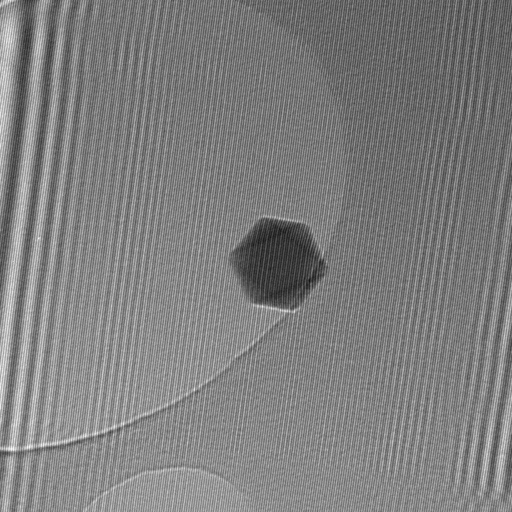
The thin lines all across the image is a direct result of the interference of the two beams. In areas with even background it closely matches a cosine function as expected. Note that the much larger parallel lines (top left) are an artifact from diffraction fringes at the edges of the biprism wire and not directly related to the phase. Let’s look at a closeup of the particle
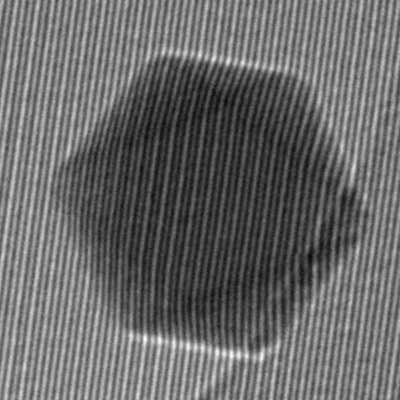
Notice how the lines are not straight everywhere. If we follow one from top to bottom, we see it bends at the top end of the particle, continues in a mostly straight line and then bends back close to its original position. This bending is directly due to the phase shift of the electron beam due to the particle - at the edges the thickness varies causing the bend, while the center of the particle is fairly even, giving straight lines. The phase shift is primarily from the electric interaction \(\phi_e\) as it tends to be stronger than \(\phi_m\).
Recovering just the phase
To separate the phase term, we turn to the trusty Fourier transform, which I wrote a bit about here. Now, as the Fourier transform is a linear operator, the transform of a sum of terms is equivalent to the sum of individually transformed terms:
\[\fourier{\Iholo} = \fourier{A_i(\vr)^2} + \fourier{A_r(\vr)^2} + \fourier{A_i(\vr)A_r(\vr)\left(e^{i(2\pi\vq_c\cdotp\vr-\phi(\vr))}+e^{-i(2\pi\vq_c\cdotp\vr-\phi(\vr))}\right)}\]With a bit of mathematical gymnastics the last term in the expression can expressed as a convolution with a delta function \(\delta(\vq\pm\vq_c)\)
\[\begin{align*} \hat{I}_\mathrm{holo} =& \hat{A}_i(\vq)^2 + \hat{A}_r(\vq)^2 \\ &+ \delta(\vq+\vq_c)*\fourier{A_i(\vr)A_r(\vr)e^{i\phi(\vr)}} \\ &+ \delta(\vq-\vq_c)*\fourier{A_i(\vr)A_r(\vr)e^{-i\phi(\vr)}} \end{align*}\]where \(*\) denotes the convolution operator. The proof of the above is left as an exercise to the reader.
It is slightly complex, but here’s what you need to take away from the above: When convolving a delta function with a fourier transform, it essentially becomes “centered” at the point where the argument of the delta function is zero; \(\delta(\mathbf{0})\). Thus if convolving with \(\delta(\vq+\vq_c)\) the center will be at \(\vq=-\vq_c\).
So now we have two amplitude terms with no phase information, \(\hat{A}_i(\vq)^2\) and \(\hat{A}_r(\vq)^2\) centered around \(\vq=(0,0)\) in the middle of the reciprocal space in the fourier transformed image. They are more or less the regular bright field image you would get without the special technique. But now we also have two phase terms, which are the complex conjugates of each other, centered at \(\vq=\vq_c\) and \(\vq=-\vq_c\) respectively. These will show up at opposite sides, away from the center of the fourier transformed image.
Visually it looks like this. Below is shown the 2D Fast Fourier Transform of the hologram image
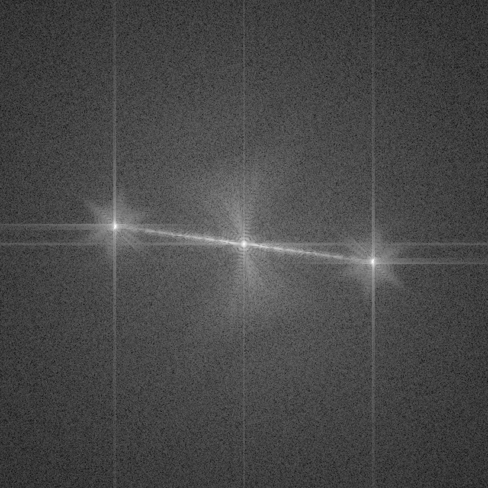
A large peak in the center with two distinct peaks away from center at opposite sides. These are the sidebands mentioned before, and the \(\vq_c\) vector is the vector pointing from the center and out to these sidebands. The visible line from the center all the way to the sideband comes from the diffraction fringes from the biprism as mentioned earlier.
Note that the Fourier transform of a real valued image results in complex values, i.e. each pixel has a real part \(\mathrm{Re}\) and imaginary part \(\mathrm{Im}\). When showing the image here, we are seeing the absolute value, or amplitude, of this complex image.
We can now select a sideband from the full image, i.e. we pick out just the term
\[\delta(\vq+\vq_c)*\fourier{A_i(\vr)A_r(\vr)e^{i\phi(\vr)}}\]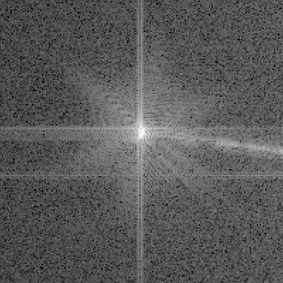
The horizontal and vertical streaks are artifacts from the edges of the image and will not affect our analysis. The center of this new image is now at \(\vq=-\vq_c\) and the convolution with the delta function becomes \(1\) leaving us with
\[\hat{I}_\mathrm{s.b.}(\vq) = \fourier{A_i(\vr)A_r(\vr)e^{i\phi(\vr)}}\]By performing an inverse Fourier transform the image is now simply
\[\Iside(\vr) = A_i(\vr)A_r(\vr)e^{i\phi(\vr)}\]We are now liberated of the other terms and we are one important step closer to isolating \(\phi(\vr)\) itself. Exciting!
Amplitude and phase of a complex number
Our sideband \(\Iside(\vr)\) is now a complex function on the exponential or polar form \(z = re^{i\varphi}\) where \(r\) is the amplitude and \(\varphi\) the phase. Mathematically we can directly read off the amplitude as \(r=A_iA_r\) and the phase of our image as \(\varphi=\phi\) but numerically our data is stored in another form.
The (Inverse) Fast Fourier Transform used to numerically perform fourier transforms gives us an image where complex numbers are in the cartesian form \(z=a+ib\), and thus each pixel has a real value \(\mathrm{Re}(z) = a\) and imaginary value \(\mathrm{Im}(z) = b\). Luckily the conversion comes from basic trigonometry. The amplitude is simply the pythagorean length of the complex number
\[r = \sqrt{a^2+b^2}\]and the phase is the angle
\[\varphi = \arctan\left(\frac{b}{a}\right)\]That’s it, we now have everything we need to recover the phase! The reconstructed phase of our particle looks like this
\[\phi(\vr) = \phi_e(\vr) + \phi_m(\vr)\]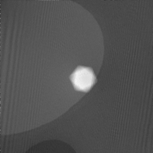
The above image (besides artifacts) is a direct image of the phase of the electron beam where it reached the detector in the microscope, reconstructed from the shown hologram. We would expect the magnetic field somewhere outside the particle, so where is it? The electric contribution \(\phi_e\) is much larger than the magnetic \(\phi_m\) so it gets a bit lost in the signal. To see it properly we still need to subtract an image of the same particle with reversed magnetic field, meaning we still have some work to do.
Summary
We’ve gone briefly through the workings of a transmission electron microscope and seen how the electron beam can be described as a wave. With a special setup in the microscope which introduces a reference wave, the interference pattern in the overlap of these waves enables us to record the phase information of the beam passing through the sample. Using some Fourier transform magic we walked through the mathematics of extracting the phase from this pattern and demonstrated it for a single particle.
The remaining work to isolate only the magnetic contribution to the phase shift is mainly computational. I continue this in the post on reconstructing holograms using Python where I walk through the code used to go from raw holograms to finished magnetic phase images.
-
Diagrams of the magnetic field around a bar magnet from Wikimedia Commons ↩
-
Takeshi Kasama, Rafal E. Dunin-Borkowski and Marco Beleggia (2011). Electron Holography of Magnetic Materials, Holography - Different Fields of Application, F. A. Ramirez (Ed.), IntechOpen, DOI: 10.5772/22366 ↩
-
Supervisors: Takeshi Kasama, Marco Beleggia, Cathrine Frandsen. On a personal note: Takeshi Kasama passed away a few years back at a much too young age. He did an amazing job as supervisor on my bachelor’s project. He had a knack for teaching and for making me “learn how to learn”, and I am grateful to have been under his guidance. He has definitely shaped my approach to science and physics and how I explain things to others, so if you like what you read send him a friendly thought! ↩
-
Strictly speaking an atom has a fuzzy undefined size, but the diameter from the Bohr model gives a useful sense of how far from the center of a hydrogen atom you are likely to find its accompanying electron. ↩
-
Since we are trying to image the weak magnetic field of our nanoparticles, the objective lens is now a Lorentz lens, as this does not generate a magnetic field at the sample. ↩
-
With acceleration voltage as \(U=\frac{E}{e}\) we have \(C_E = \left(\frac{2\pi}{\lambda}\right) \left(\frac{E+E_0}{E(E+2E_0)}\right)\) where \(\lambda\) is the relativistic electron wavelength and \(E_0\) the rest mass energy of the electron. ↩
-
There are also other ways of removing the electric phaseshift \(\phi_e\), such as directly simulating \(\phi_e\) from detailed sample information and subtracting that. It can also be useful on its own, e.g. for accurate measurements of particle thickness, but we will not consider this for now. ↩
-
Using some identities of complex exponentials we can also write the phase term as a cosine term \(A_i(\vr)A_r(\vr) \cos\left[2\pi\vq_c\cdot\vr+\phi(\vr)\right]\). These sinusoidal interference fringes are what we directly measure in the raw hologram. ↩
-
Take a look at Agar scientific for some example images. ↩